Chapter 7 Mixed Model

7.1 introduction

This is summary tutor of linear mixed model. The main reference is https://ourcodingclub.github.io/tutorials/mixed-models/

The data have different hierarchical or grouping characteristics like some patients from different hospitals. In that situation, the stratification analysis is most common methods to figure out exact relationship. However, the lack of power with limit sample size issue came from stratification analysis. So, When those factors all were putted in together, the mixed models were needed. Here, I summary linear mixed models here. In current case summary, We will used covid19 data from 16th countries. The group is country level and the interesting relationship is regarded on individual economic activity and psychological symptoms. The original data are own to Laura, PH.D, Michigan university.

7.2 data step 1

import library

rm(list=ls())
library(tidyverse)
library(htmlTable)
library(readxl)
library(ggrepel)
#library(doMC)
#registerDoMC(31)
library(data.table)
library(DT)
library(plotly)
library(readr)
library(readxl)
library(gridExtra)
library(broom);library(broom.mixed)

7.3 load data of Int and Korea

data import of international and korea

#new laura data Dec 2020
#international and korea data
covid = read_csv('data/covid/covid.csv')
kr_d  <- read_xlsx('data/covid/kr_data.XLSX', sheet = 1)
cbook <- read_xlsx('data/covid/code_book.xlsx')
# human development index
hdi = read_csv('data/covid/hdi.csv') %>% 
  setNames(c('rank', 'country', 'y2019', 'country_1'))

look up tabel for country name and number

country_lkup <- data.frame(country = c(1, 16, 31, 36,65, 75, 79, 104, 136, 137, 143, 156, 168, 172, 173, 179, 183, 192), 
                           country_c = c(
                             "USA", "Belarus", "Canada", "China", 
                             "German", "Hong Kong", "Indonesia", 
                             "Malaysia", "Philippines", "Poland", 
                             "Rusia", "Singapore", "Sweden", 
                             "Thailand", "Taiwan", "Turkey", 
                             "Ukraine", "Vietnam"
                             
                           ))

overview of codebook

cbook %>% datatable()

Korea Data step for value and variable standardization

kr_d1 <- kr_d %>%
      select('IDnum' = No, 'age' = SQ2, 'gender' = SQ1, 'Education'  = DQ1,
             contains('DQ2'), # employment status
             'EmoDep'  = Q18_2, # for int Q36_2 how much have you feeling
             'EmoAnx'  = Q18_3, # for int Q36_3
             'ChrDep'  = Q21_10, # for int Q40_17
             'ChrAnx'  = Q21_11, # for int Q40_18
             'ToDepAnx'= Q22_5, # for int Q41_5, 
             'dfLossJob' = Q10_10, # for int Q26_9,
             'dfReduIcm' = Q10_3, # for int Q26_3, 
             'dfIncAnx'  = Q10_5 # for int Q26_5  
             ) %>%
  mutate(country = 200, country_c = 'South Korea') %>%
  map_if(is.numeric, ~ifelse(is.na(.x), 0, .x) ) %>%
 as.data.frame()

international data mutate

international Data step

int_d1 <- covid %>%
      mutate('age' = 2020 - Q79) %>%
     mutate(IDnum = row_number()) %>%
      select(IDnum,
             'age',
             'gender' = Q10, 'Education'  = Q80,
             contains('Q94'), # employment status
             'EmoDep'  = Q36_2, 
             'EmoAnx'  = Q36_3,
             'ChrDep'  = Q40_17,
             'ChrAnx'  = Q40_18,
             'ToDepAnx'= Q41_5, 
             'dfLossJob' = Q26_9,
             'dfReduIcm' = Q26_3, 
             'dfIncAnx'  = Q26_5, 
             'country' = Q2
             ) %>%
   
   left_join(country_lkup,  by = c('country')) %>%
   select(-Q94_18, -Q94_19)

Harmonizing Variable name between Korea and International Data

em_lkup = tibble(
  'kr' = c('DQ2_1', 'DQ2_2', 'DQ2_3', 'DQ2_4', 'DQ2_5', 'DQ2_6', 'DQ2_7', 
           'DQ2_8','DQ2_9','DQ2_10','DQ2_11','DQ2_12','DQ2_13','DQ2_14'), 
  'int' =c('Q94_9', 'Q94_2',    'Q94_3',    'Q94_4',    'Q94_7',    'Q94_8',    'Q94_5',    'Q94_12',   'Q94_14',   'Q94_15',   'Q94_1',    'Q94_6',    'Q94_16',   'Q94_17')

)

kr_d2<- kr_d1 %>%
plyr::rename(setNames(em_lkup$int, em_lkup$kr)) # change kr variable names to int variable names. 

# colnames(kr_d2)   == colnames(int_d1) # it returns TRUE value for all col names

7.4 data merge

mm <- rbind(int_d1, kr_d2)
nrow(mm)

## [1] 19270

mm <- mm %>% na.omit(age)
nrow(mm) 

## [1] 16942

data mutate

krtoint = function(x) {
  x = ifelse(x<4, x+4, x)
}
logictozero= function(x){
  x = as.numeric(x != 0)
}
mm1 <-mm %>%
  filter(age >20 & age <65) %>%
  filter(gender %in% c(1, 2)) %>%
  filter(!((EmoDep ==-99)|(EmoAnx ==-99)|(dfLossJob==-99)|(Q94_3==-99)|(Q94_4 ==-99)))%>%
  mutate (dfLossJob = ifelse(dfLossJob ==10, 1, dfLossJob)) %>%
  mutate (Q94_3 = ifelse(!Q94_3 == 0, 1, 0)) %>%
  mutate (Q94_4 = ifelse(!Q94_4 == 0, 1, 0))
  
mm12<- mm1 %>%
  mutate(EmoDep =krtoint(EmoDep), 
         EmoAnx =krtoint(EmoAnx), 
         ToDepAnx=ifelse(ToDepAnx == 3, 1, 0)) %>%
  select(-c('ChrDep', 'ChrAnx', 'dfLossJob','dfReduIcm','dfIncAnx' ))

mm13 <- mm1 %>%
  select(c('ChrDep', 'ChrAnx', 'dfLossJob','dfReduIcm','dfIncAnx' )) %>%
  lapply(., logictozero) %>%
  data.frame()

mm2 <- cbind(mm12, mm13)

  


mm3 <- mm2 %>%
  mutate(EcLoss       = ifelse(Q94_3 !=0 | Q94_4!=0, 1, 0)) %>%
  mutate(EcLossUnSafe = ifelse(Q94_4!=0, 1, 0)) %>%
  mutate(agegp = cut(age, breaks = c(-Inf, (5:13)*5, +Inf))) %>%
  mutate(agegp2 = as.numeric(agegp)) %>%
  mutate(gender = ifelse(gender ==1, 'Men', 'Women')) %>%
  mutate(Edugp = factor(Education, levels = c(1, 2, 3, 4, 5, 6), 
                        labels = c("Middle or less", "High", "Colleage", 
                                   "University", "Graduate Sc", "Doctoral or more"))) %>%
  mutate(EcLossAll = EcLoss + dfLossJob ) %>%
  mutate(TotalDepAnx = ifelse(EmoDep ==7 | EmoAnx ==7, 1, 0))
  #mutate(TotalDepAnx= as.numeric((as.numeric(EmoDep ==7) + as.numeric(EmoAnx ==7))) !=0)

create basic matrix for visualization (NA as zero)

mm4 <- mm3 %>%
    mutate(agegp3 = ifelse(age <=40, '≤40', '>40')) %>%
    mutate(agegp3 = factor(agegp3, levels=c('≤40', '>40'))) %>%
    filter(Education %in% c(1:6)) %>%
    mutate(edugp = ifelse(Education %in% c(1, 2), 1, # high school or less
                        ifelse(Education %in% c(3),2, # college
                               ifelse(Education %in% c(4), 3, 4)))) %>% # university (5, 6) Graduate school
 mutate(edugp2 = ifelse(Education %in% c(1, 2, 3), 1, 2)) %>%
 mutate(EcLossAllgp = ifelse(EcLossAll ==0, 0, 1)) #%>%
#filter(!country %in% c(16, 173))

bm1<-crossing(
    'gender'=unique(mm4$gender),
    'country_c'=unique(mm4$country_c),
    'edugp'=unique(mm4$edugp),
    'edugp2'=unique(mm4$edugp2),
    'agegp2'=unique(mm4$agegp2), 
    'agegp3'=unique(mm4$agegp3),
    'EcLossAllgp'=unique(mm4$EcLossAllgp), 
    'TotalDepAnx' = unique(mm4$TotalDepAnx)
)

mm4.0 = mm4 %>%
  left_join(hdi %>% filter(!is.na(country_1)) %>%
  rename(country_source = country,
         country=country_1   ), by = c('country')) %>%
  mutate(y2019 = ifelse(country_c =='South Korea', 0.916, y2019))

7.5 Data analysis start

7.5.1 job loss due to COVID19, psychological aggravation according to Gender

due to covid vary by country basic static for job loss prevalence across country and genders.

fig1 <- mm4 %>%
  group_by(country_c, gender) %>%
  count(EcLossAllgp) %>%
  mutate(prob = n/sum(n)) %>%
  filter(EcLossAllgp == 1 ) %>%
  ggplot(aes(x = gender, y = prob, fill = gender)) +
  geom_bar(stat = "identity")+
  xlab("")+
  ylab("Job loss due to COVID19")+
  scale_y_continuous(labels = function(x) paste0(x*100, "%"))+
  facet_wrap(country_c ~., nrow = 3) +
  theme_minimal()+
  theme(text = element_text(size=17))+
  theme(legend.position = c(.92, .1))

fig2 <- mm4 %>%
  group_by(country_c, gender) %>%
  count(TotalDepAnx) %>%
  mutate(prob = n/sum(n)) %>%
  filter(TotalDepAnx == 1 ) %>%
  ggplot(aes(x = gender, y = prob, fill = gender)) +
  geom_bar(stat = "identity")+
  ylab("Psychological aggravation due to COVID19")+
  xlab('Gender')+
  scale_y_continuous(labels = function(x) paste0(x*100, "%"))+
  facet_wrap(country_c ~., nrow = 3) +
  theme_minimal()+
  theme(text = element_text(size=17))+
  theme(legend.position = c(.92, .1))

Save total figure

ggsave(arrangeGrob(fig1, fig2, ncol = 1), file ='results/covid/figtotal.png', dpi = 300, width = 10, height =14)
ggsave(arrangeGrob(fig1, fig2, ncol = 1), file ='results/covid/tiff/figtotal.tiff', dpi = 300, width = 10, height =14)

7.5.2 job loss, psychological aggravation according to age group

fig3 <- mm4.0 %>%
  #filter(!country %in% c(16, 173)) %>%
  group_by(country_c, gender, agegp2) %>%
  count(EcLossAllgp) %>%
  mutate(prob = n/sum(n)) %>%
  filter(EcLossAllgp == 1) %>%
  ggplot(aes(x = agegp2, y = prob, color = gender)) +
  geom_point(aes(size = n), alpha = 0.2, show.legend = FALSE) +
  geom_smooth(method = 'loess', span =0.9,  se=FALSE) + 
   ylab("Job loss due to COVID19")+
    scale_y_continuous(labels = function(x) paste0(x*100, "%"))+
  theme_minimal() +
  xlab("")+
  labs(color = "Gender") +
  facet_wrap(country_c~., nrow =3)+
  theme(legend.position = c(.92, .1))+
  theme(text = element_text(size=17))+
  scale_x_continuous(breaks = c(2,4,6,8), labels = c(30,40,50,60))

fig4 <- mm4.0 %>%
  #filter(!country %in% c(16, 173)) %>%
  group_by(country_c, gender, agegp2) %>%
  count(TotalDepAnx) %>%
  mutate(prob = n/sum(n)) %>%
  filter(TotalDepAnx == 1) %>%
  ggplot(aes(x = agegp2, y = prob, color = gender)) +
  geom_point(aes(size = n), alpha = 0.2, show.legend = FALSE) +
  geom_smooth(method = 'loess', span =0.9,  se=FALSE) + 
   ylab("Psychological aggravation due to COVID19")+
    scale_y_continuous(labels = function(x) paste0(x*100, "%"))+
  theme_minimal() +
  xlab("Age (size = number of respondents)") +
  labs(color = "Gender") +
  facet_wrap(country_c~., nrow =3)+
  theme(legend.position = c(.92, .1))+
  theme(text = element_text(size=17))+
  scale_x_continuous(breaks = c (2,4,6,8), labels = c(30,40,50,60))

save figures

#figtotal2 <- grid.arrange(fig3, fig4, ncol = 1)
ggsave(arrangeGrob(fig3, fig4, ncol = 1), file ='results/covid/figtotal2.png', dpi = 300, width = 10, height =14)
ggsave(arrangeGrob(fig3, fig4, ncol = 1), file ='results/covid/tiff/figtotal2.tiff', dpi = 300, width = 10, height =14)

7.6 job loss, psychological aggravation according to Education level

fig5 <- mm4.0 %>%
  group_by(edugp, country_c, gender) %>%
  count(EcLossAllgp ) %>%
  mutate(prob = n/sum(n)) %>%
  filter(EcLossAllgp  == 1) %>%
  ggplot(aes(x = edugp, y = prob, color = gender)) +
  geom_smooth(method = 'loess', span =0.9, se = FALSE) +
  scale_x_continuous(labels=c("1" = "≤H", "2" = "C",
                            "3" = "U", "4" = "G")) +
  theme_minimal() + 
  labs(color = "Gender") +
  ylab("Job Loss due to COVID19") +
  xlab("")+
  facet_wrap(country_c ~., nrow = 3)+
  theme(text = element_text(size=17))+
  theme(legend.position = c(.92, .1))

# mm4 %>%
#   count(TotalDepAnx)
fig6 <- mm4.0 %>%
  group_by(edugp, country_c, gender) %>%
  count(TotalDepAnx ) %>%
  mutate(prob = n/sum(n)) %>%
  filter(TotalDepAnx  == 1  ) %>%
  ggplot(aes(x = edugp, y = prob, color = gender)) +
  geom_smooth(method = 'loess', span =0.9, se = FALSE) +
  scale_x_continuous(labels=c("1" = "≤H", "2" = "C",
                            "3" = "U", "4" = "G")) +
  theme_minimal() + 
  ylab("Psychological aggravation due to COVID19") +
  scale_y_continuous(labels = function(x) paste0(x*100, "%"))+
  xlab("H = high school, C = college, U = university, G = graduate ") +
  labs(color = "Gender") +
  facet_wrap(country_c ~., nrow = 3)+
  theme(text = element_text(size=17))+
  theme(legend.position = c(.92, .1))

save figure

#figtotal3 <- grid.arrange(fig5, fig6, ncol = 1)
ggsave(arrangeGrob(fig5, fig6, ncol = 1), file ='results/covid/figtotal3.png', dpi = 300, width = 10, height =14)
ggsave(arrangeGrob(fig5, fig6, ncol = 1), file ='results/covid/tiff/figtotal3.tiff', dpi = 300, width = 10, height =14)

knitr::include_graphics('results/covid/figtotal3.png')

7.6.1 Depression status according job loss status

basic statistic for DepAnx prevalence across country and genders.

7.7 association

(ref: https://cran.r-project.org/web/packages/sjPlot/vignettes/tab_model_estimates.html)

if (!require('sjPlot')) install.packages('sjPlot')
if (!require('sjmisc')) install.packages('sjmisc')
if (!require('sjlabelled')) install.packages('sjlabelled')
library(sjPlot);library(sjmisc);library(sjlabelled)

countries <- c("Taiwan","USA", "Belarus", "Canada", "China", 
                             "German", "Hong Kong", "Indonesia", 
                             "Malaysia", "Philippines", "Poland", 
                             "Rusia", "Singapore", "Sweden", 
                             "Thailand", "South Korea", "Turkey", 
                             "Ukraine", "Vietnam")

mm4.1 <- mm4.0 %>% 
  mutate(TotalDepAnx = factor(TotalDepAnx, levels =c(0,1)),
         EcLossAllgp = factor(EcLossAllgp, levels =c(0,1)),
         gender      = factor(gender, levels =c('Men', 'Women')),
         edugp2       = factor(edugp2, levels = c(1,2)),
         country_c   = factor(country_c, levels= countries))

regression model

mod1 = mm4.1 %>%
    glm(family = binomial, 
       formula = TotalDepAnx ~ EcLossAllgp) 
mod2 = mm4.1 %>%
    glm(family = binomial, 
       formula = TotalDepAnx ~ EcLossAllgp + age + gender + edugp2) 
mod3 = mm4.1 %>%
    glm(family = binomial, 
       formula = TotalDepAnx ~ EcLossAllgp + age + gender + edugp2 + 
         relevel(as.factor(country_c), ref = 'Taiwan') )

tab_model(mod1, mod2, mod3)

	TotalDepAnx			TotalDepAnx			TotalDepAnx
Predictors	Odds Ratios	CI	p	Odds Ratios	CI	p	Odds Ratios	CI	p
(Intercept)	1.34	1.29 – 1.39	<0.001	1.37	1.19 – 1.58	<0.001	0.88	0.72 – 1.09	0.257
EcLossAllgp [1]	1.65	1.51 – 1.79	<0.001	1.64	1.51 – 1.79	<0.001	1.55	1.42 – 1.70	<0.001
age				0.99	0.99 – 0.99	<0.001	0.99	0.99 – 0.99	<0.001
gender [Women]				1.33	1.24 – 1.42	<0.001	1.34	1.25 – 1.43	<0.001
edugp2 [2]				1.34	1.24 – 1.43	<0.001	1.28	1.19 – 1.39	<0.001
relevel(country c, ref = “Taiwan”)USA							1.73	1.41 – 2.14	<0.001
relevel(country c, ref = “Taiwan”)Canada							1.42	1.15 – 1.75	0.001
relevel(country c, ref = “Taiwan”)China							1.33	1.10 – 1.61	0.003
relevel(country c, ref = “Taiwan”)German							0.94	0.76 – 1.16	0.567
relevel(country c, ref = “Taiwan”)Hong Kong							1.22	0.97 – 1.53	0.093
relevel(country c, ref = “Taiwan”)Indonesia							2.48	2.02 – 3.04	<0.001
relevel(country c, ref = “Taiwan”)Malaysia							1.02	0.83 – 1.25	0.847
relevel(country c, ref = “Taiwan”)Philippines							1.35	1.10 – 1.66	0.004
relevel(country c, ref = “Taiwan”)Poland							3.01	2.44 – 3.73	<0.001
relevel(country c, ref = “Taiwan”)Singapore							1.77	1.39 – 2.25	<0.001
relevel(country c, ref = “Taiwan”)Sweden							0.82	0.66 – 1.02	0.076
relevel(country c, ref = “Taiwan”)Thailand							2.98	2.42 – 3.67	<0.001
relevel(country c, ref = “Taiwan”)South Korea							2.72	2.23 – 3.33	<0.001
relevel(country c, ref = “Taiwan”)Turkey							3.35	2.72 – 4.15	<0.001
relevel(country c, ref = “Taiwan”)Ukraine							1.20	0.98 – 1.47	0.072
relevel(country c, ref = “Taiwan”)Vietnam							1.89	1.54 – 2.33	<0.001
Observations	14243			14243			14243
R2 Tjur	0.009			0.022			0.065

summay stat of each models.

7.7.1 mixed model

if(!require(lme4)) install.packages('lme4');library(lme4)

first mixed model

mm4.2 = mm4.1 %>%
  mutate(country_c2 = relevel(as.factor(country_c), ref = 'Taiwan') ) %>%
  mutate(TotalDepAnx2 = as.numeric(TotalDepAnx)) %>%
  mutate(EcLossAllgp2 = as.numeric(EcLossAllgp)) %>%
  mutate(edugp3 = as.numeric(edugp2)) %>%
  mutate(age2 = as.numeric(age)) %>%
  mutate(gender2 = as.numeric(gender)) 

mixed.lmer = lmer(TotalDepAnx2 ~ EcLossAllgp2 + age + edugp + gender+ 
                    (1|country_c2), data=mm4.2)
summary(mixed.lmer)

## Linear mixed model fit by REML ['lmerMod']
## Formula: TotalDepAnx2 ~ EcLossAllgp2 + age + edugp + gender + (1 | country_c2)
##    Data: mm4.2
## 
## REML criterion at convergence: 19305.2
## 
## Scaled residuals: 
##     Min      1Q  Median      3Q     Max 
## -1.8980 -1.0808  0.5415  0.8399  1.5079 
## 
## Random effects:
##  Groups     Name        Variance Std.Dev.
##  country_c2 (Intercept) 0.01083  0.1040  
##  Residual               0.22546  0.4748  
## Number of obs: 14243, groups:  country_c2, 17
## 
## Fixed effects:
##                Estimate Std. Error t value
## (Intercept)   1.4655134  0.0346770  42.262
## EcLossAllgp2  0.0963579  0.0100154   9.621
## age          -0.0021919  0.0003372  -6.501
## edugp         0.0228408  0.0040361   5.659
## genderWomen   0.0653560  0.0080437   8.125
## 
## Correlation of Fixed Effects:
##             (Intr) EcLsA2 age    edugp 
## EcLssAllgp2 -0.409                     
## age         -0.459  0.090              
## edugp       -0.357  0.064  0.057       
## genderWomen -0.164  0.027  0.103 -0.007

#qqnorm(resid(mixed.lmer))

mixed.lmer2 = lmer(TotalDepAnx2 ~ EcLossAllgp + age2 +
                    (1|edugp3)+ (1|country_c2/gender2), data=mm4.2)
summary(mixed.lmer2)

## Linear mixed model fit by REML ['lmerMod']
## Formula: 
## TotalDepAnx2 ~ EcLossAllgp + age2 + (1 | edugp3) + (1 | country_c2/gender2)
##    Data: mm4.2
## 
## REML criterion at convergence: 19288.9
## 
## Scaled residuals: 
##     Min      1Q  Median      3Q     Max 
## -1.9338 -1.0857  0.5291  0.8523  1.5039 
## 
## Random effects:
##  Groups             Name        Variance Std.Dev.
##  gender2:country_c2 (Intercept) 0.003000 0.05477 
##  country_c2         (Intercept) 0.008937 0.09453 
##  edugp3             (Intercept) 0.001716 0.04142 
##  Residual                       0.224888 0.47422 
## Number of obs: 14243, groups:  
## gender2:country_c2, 34; country_c2, 17; edugp3, 2
## 
## Fixed effects:
##               Estimate Std. Error t value
## (Intercept)   1.646672   0.041157  40.010
## EcLossAllgp1  0.095570   0.010010   9.548
## age2         -0.002198   0.000338  -6.503
## 
## Correlation of Fixed Effects:
##             (Intr) EcLsA1
## EcLssAllgp1 -0.084       
## age2        -0.343  0.091

#qqnorm(resid(mixed.lmer2))

mixed.lmer3 = lmer(TotalDepAnx2 ~ EcLossAllgp + age2 + edugp2+
                  (1+TotalDepAnx2|country_c2/gender2), data=mm4.2)
summary(mixed.lmer3)

## Linear mixed model fit by REML ['lmerMod']
## Formula: TotalDepAnx2 ~ EcLossAllgp + age2 + edugp2 + (1 + TotalDepAnx2 |  
##     country_c2/gender2)
##    Data: mm4.2
## 
## REML criterion at convergence: -394555.3
## 
## Scaled residuals: 
##        Min         1Q     Median         3Q        Max 
## -3.702e-06 -2.610e-07  1.009e-07  3.772e-07  2.663e-06 
## 
## Random effects:
##  Groups             Name         Variance  Std.Dev.  Corr 
##  gender2:country_c2 (Intercept)  8.457e-06 2.908e-03      
##                     TotalDepAnx2 2.315e-03 4.812e-02 -0.86
##  country_c2         (Intercept)  5.900e-05 7.681e-03      
##                     TotalDepAnx2 4.791e-05 6.922e-03 0.68 
##  Residual                        4.745e-14 2.178e-07      
## Number of obs: 14243, groups:  gender2:country_c2, 34; country_c2, 17
## 
## Fixed effects:
##               Estimate Std. Error t value
## (Intercept)  1.431e-02  1.932e-03   7.408
## EcLossAllgp1 1.691e-14  4.623e-09   0.000
## age2         1.732e-15  1.562e-10   0.000
## edugp22      1.311e-14  4.080e-09   0.000
## 
## Correlation of Fixed Effects:
##             (Intr) EcLsA1 age2 
## EcLssAllgp1 0.000              
## age2        0.000  0.085       
## edugp22     0.000  0.067  0.069
## optimizer (nloptwrap) convergence code: 0 (OK)
## unable to evaluate scaled gradient
## Model failed to converge: degenerate  Hessian with 1 negative eigenvalues

#qqnorm(resid(mixed.lmer2))

make region variable, humain devepin index and .. stratification anaysis. (Asia vs non-Asia or …) deveolping index ..

7.7.2 mixed model with human develop index stratification

agu1 <- read_csv('data/covid/covid_agu1.csv')

lab_mm <- mm4.0 %>%
  left_join(agu1, by = 'country_c') %>%
  mutate(inc_aug = c_case_agu1 / population *100000, 
         dth_aug = c_death_agu1/ population *100000) %>%
  group_by(country_c, gender) %>%
  summarize(hdi = mean(y2019), 
            Psycho = mean(TotalDepAnx ==1), 
            ecl = mean(EcLossAll !=0),
            inc = mean(inc_aug)) 

lab_mm%>%
  ggplot(aes(x = hdi, y = ecl, color = inc)) +
  geom_point() +
  theme_classic()+
  xlab("Human Devlopment Index") +
  #ylab("prevalance of Psychological Symptoms") +
  ylab("prevalance of Economic Loss due to COVID19") + 
  #ylim(c(-0.1, 1)) + #xlim(c(2, 4)) + 
  geom_label_repel(aes(label = country_c), 
                   fill = NA, # 투명하게 해서 겹쳐도 보이게
                   alpha =1, size = 3, # 작게
                   box.padding = 0.4,  # 분별해서
                   segment.size =0.1,  # 선 
                   force = 2)      +    # 이것은 무엇일까요?
   theme_minimal() +
  geom_smooth(method = 'lm', formula = y ~ poly(x,2), se=FALSE) +
  #geom_smooth( se=FALSE) +
  facet_wrap(gender~.) +
  guides(color = "none")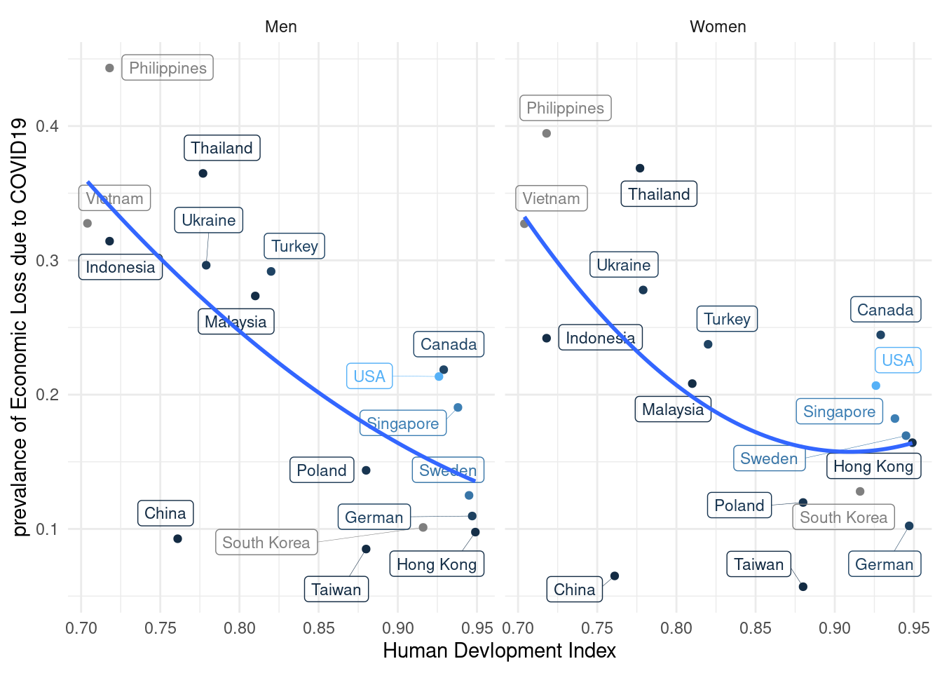

mixed.lmer4 = lmer(TotalDepAnx2 ~ EcLossAllgp2 + age2 + 
                  (1|country_c), data=mm4.2 %>% filter(edugp2 ==2))
summary(mixed.lmer4)

## Linear mixed model fit by REML ['lmerMod']
## Formula: TotalDepAnx2 ~ EcLossAllgp2 + age2 + (1 | country_c)
##    Data: mm4.2 %>% filter(edugp2 == 2)
## 
## REML criterion at convergence: 12714
## 
## Scaled residuals: 
##     Min      1Q  Median      3Q     Max 
## -1.8649 -1.1252  0.5519  0.8157  1.4511 
## 
## Random effects:
##  Groups    Name        Variance Std.Dev.
##  country_c (Intercept) 0.01124  0.1060  
##  Residual              0.22338  0.4726  
## Number of obs: 9436, groups:  country_c, 17
## 
## Fixed effects:
##                Estimate Std. Error t value
## (Intercept)   1.6157913  0.0351975  45.906
## EcLossAllgp2  0.0874493  0.0123267   7.094
## age2         -0.0028828  0.0004268  -6.754
## 
## Correlation of Fixed Effects:
##             (Intr) EcLsA2
## EcLssAllgp2 -0.455       
## age2        -0.518  0.072

#qqnorm(resid(mixed.lmer2))

mod3 = mm4 %>% glm(family = binomial, formula = TotalDepAnx ~ EcLossAllgp + age + gender + edugp2 + relevel(as.factor(country_c), ref = ‘Taiwan’) )

mixed.lmer1 = lmer(TotalDepAnx2 ~ EcLossAllgp2 + age + edugp + gender+ 
                    (1|country_c2), data=mm4.2 %>% filter(y2019 >0.9))
summary(mixed.lmer1)

## Linear mixed model fit by REML ['lmerMod']
## Formula: TotalDepAnx2 ~ EcLossAllgp2 + age + edugp + gender + (1 | country_c2)
##    Data: mm4.2 %>% filter(y2019 > 0.9)
## 
## REML criterion at convergence: 6860.8
## 
## Scaled residuals: 
##     Min      1Q  Median      3Q     Max 
## -1.8989 -1.0078  0.5255  0.8818  1.5447 
## 
## Random effects:
##  Groups     Name        Variance Std.Dev.
##  country_c2 (Intercept) 0.01017  0.1008  
##  Residual               0.23064  0.4802  
## Number of obs: 4962, groups:  country_c2, 7
## 
## Fixed effects:
##               Estimate Std. Error t value
## (Intercept)   1.411453   0.055829  25.282
## EcLossAllgp2  0.127543   0.018872   6.758
## age          -0.002507   0.000560  -4.477
## edugp         0.014514   0.006520   2.226
## genderWomen   0.102722   0.013814   7.436
## 
## Correlation of Fixed Effects:
##             (Intr) EcLsA2 age    edugp 
## EcLssAllgp2 -0.435                     
## age         -0.513  0.107              
## edugp       -0.343 -0.006  0.090       
## genderWomen -0.194 -0.015  0.117  0.064

mixed.lmer2 = lmer(TotalDepAnx2 ~ EcLossAllgp2 + age + edugp + gender+ 
                     (1|country_c2), data=mm4.2 %>% filter(y2019 <=0.9 & y2019 >=0.8))
mixed.lmer3 = lmer(TotalDepAnx2 ~ EcLossAllgp2 + age + edugp + gender+ 
                     (1|country_c2), data=mm4.2 %>% filter(y2019 <=0.8))

hdi0.9 = summary(mixed.lmer1)$coefficient[2, 1] %>% exp()
hdi0.8 = summary(mixed.lmer2)$coefficient[2, 1] %>% exp()
hdi0.7 = summary(mixed.lmer3)$coefficient[2, 1] %>% exp()
hdi0.9ci = confint(mixed.lmer1)[4, ] %>% exp()
hdi0.8ci = confint(mixed.lmer2)[4, ] %>% exp()
hdi0.7ci = confint(mixed.lmer3)[4, ] %>% exp()
hdi0.9ci

##    2.5 %   97.5 % 
## 1.094813 1.178854

tibble(c(hdi0.9, hdi0.9ci), 
c(hdi0.8, hdi0.8ci), 
c(hdi0.7, hdi0.7ci)) %>%
  setNames(c('OR', 'LL', 'UL')) %>%
  mutate(HDI = c('>0.9', '>0.8', '<0.8')) %>%
  select(HDI, OR, LL, UL)

## # A tibble: 3 × 4
##   HDI      OR    LL    UL
##   <chr> <dbl> <dbl> <dbl>
## 1 >0.9   1.14  1.09  1.09
## 2 >0.8   1.09  1.04  1.06
## 3 <0.8   1.18  1.13  1.12