Chapter 10 Basic plot with R
Now this is a basic R visualization tutorial using GGPLOT2 and some related libraries. It includes basic plotting principles and setup options. At the end of the tutorial, you will have a working visualization example for Data Explorer.
10.1 ggplot basic
Before drawing basic tables and graphs, let’s take a look at the most used package, ggplot2. Let’s practice ggplot2 using the built-in data iris.
library(tidyverse)
data(iris)
The main syntax for ggplot2 are included by axis and layer. Let’s Take It from the begging.
10.1.1 axis
2-denominational plot needs 3 components of data, axis,layer. First we draw x-axis and y-axis, and putting information into that using layer.
iris %>% # data what we used
  ggplot(aes(x = Sepal.Length, y = Sepal.Width))
In this way, the X and Y axes were created. Let’s change the axis names to xlab, ylab and use ggtitle to change the title.
iris %>%
  ggplot(aes(x = Sepal.Length, y = Sepal.Width)) +
  xlab("sepal length") + ylab("sepal width") +
  ggtitle("Iris flow and its characteristics")
10.1.2 layer, geom_x()
Layers are what you want to put inside the frame. geom_x() format. _x() can be points, lines, smoothing, histograms, densities, boxplots, and bars.
| geom_x() | contents |
|---|---|
| geom_point() | scatter plot |
| geom_line() | line plot |
| geom_smooth() | prediction line |
| geom_histogram() | histogram |
| geom_density() | density line |
| geom_boxplot() | boxplot plot |
| geom_bar() | bar chart |
10.1.3 geom_point()
This is the most basic scatterplot. Plot Sepal.Length on the x-axis and Sepal.Width on the y-axis. The layer to use in this case is geom_point().
iris %>%
  ggplot(aes(x=Sepal.Length, y = Sepal.Width)) +
  geom_point()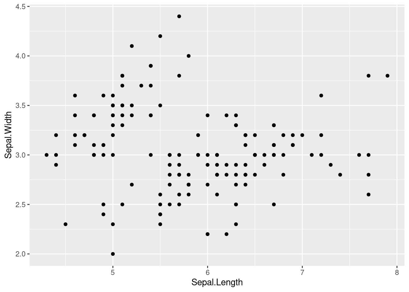
You can put a description here using xlalb and ylab. Create a title using ggtitle(). .
iris %>%
ggplot(aes(x = Sepal.Length, y = Sepal.Width)) +
xlab("Sepal length") +
ylab("Sepal width") +
ggtitle(" Type of iris according to sepal lenght and width") +
geom_point()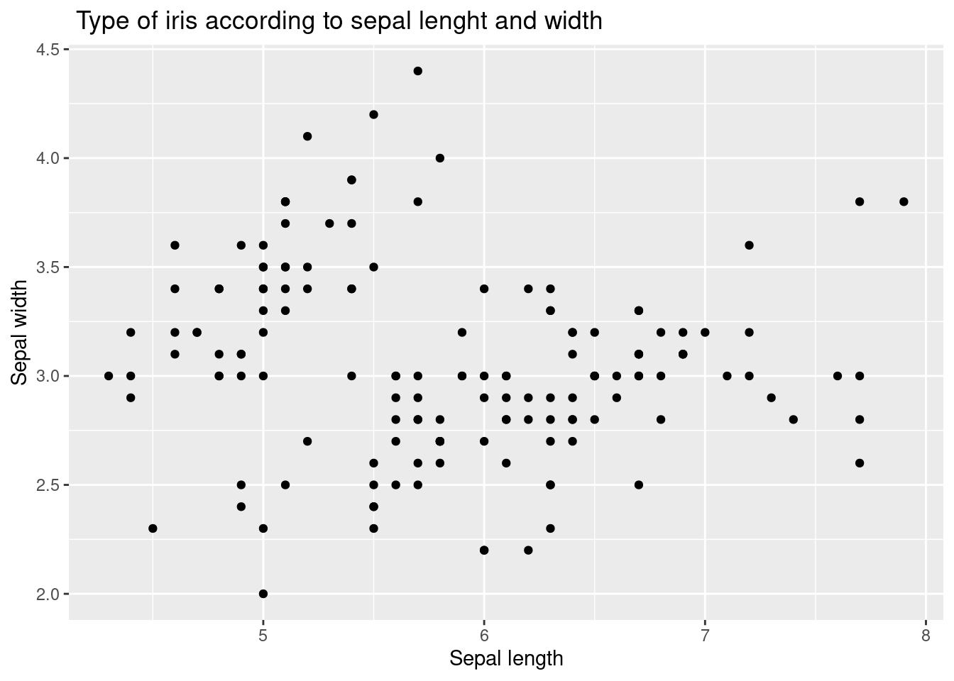 Let’s go further. There is no interpretation in scatter plots. At this time, we will use different colors for each type of iris. We will create a frame by putting color = Species inside aes( ).
iris %>%
ggplot(aes(x = Sepal.Length, y = Sepal.Width,
color = Species)) +
xlab("Sepal length") +
ylab("Sepal width") +
ggtitle(" Type of iris according to sepal lenght and width") +
geom_point()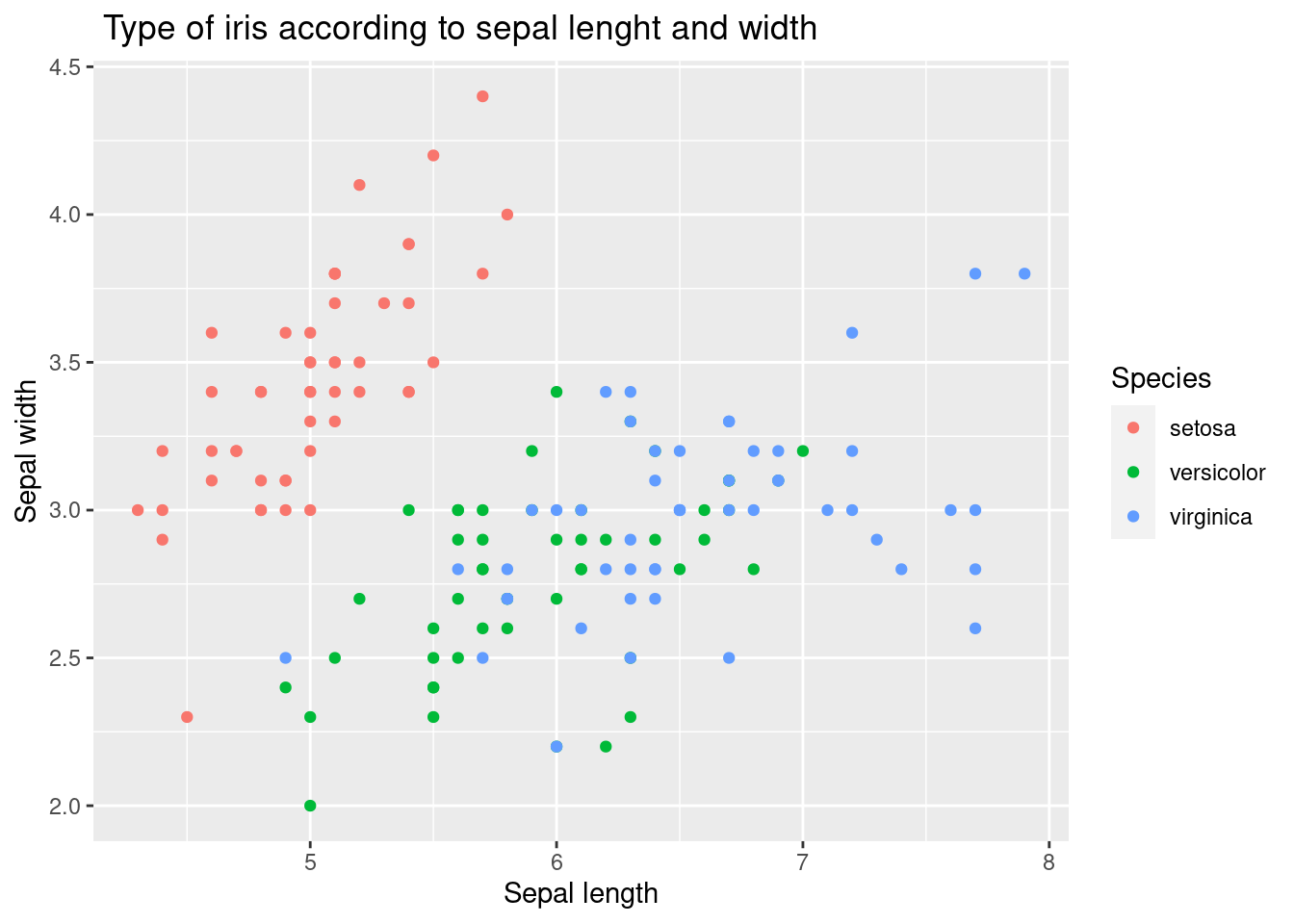 How about it? A little bit better. This time, we will add a trend line geom_smooth() to examine the relationship between sepal length and width by type. Also try adding geom_line() . It is omitted here because it is not logically useful.
10.1.4 geom_smooth()
iris %>% #
  ggplot(aes(x = Sepal.Length, y = Sepal.Width,
             color = Species)) +
  xlab("Sepal length") +
  ylab("Sepal width") +
  ggtitle(" Type of iris according to sepal lenght and width") +
  geom_point() +
geom_smooth() 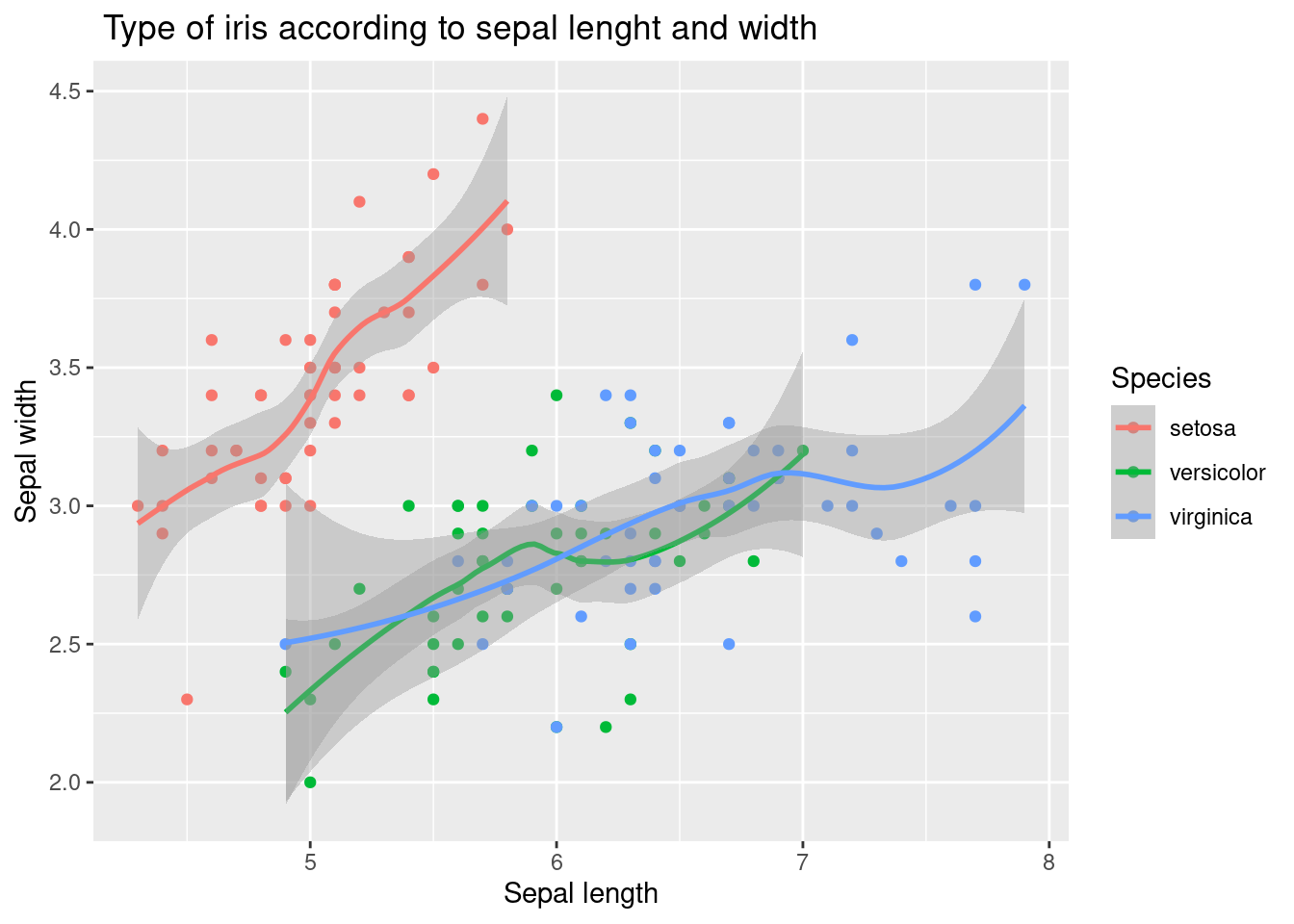
The following code demonstrated example of adding a linear trend line as well as polynomial line.
iris %>%
  ggplot(aes(x = Sepal.Length, y = Sepal.Width,
             color = Species)) +
  xlab("Sepal length") +
  ylab("Sepal width") +
  ggtitle(" Type of iris according to sepal lenght and width") +
  geom_point() +
  geom_smooth(method = 'lm', formula = y ~ poly(x, 5), se = FALSE, linetype = 1) + # how abou se = TRUE
geom_smooth(method = 'lm', formula = y ~ x, se = FALSE, linetype = 2) 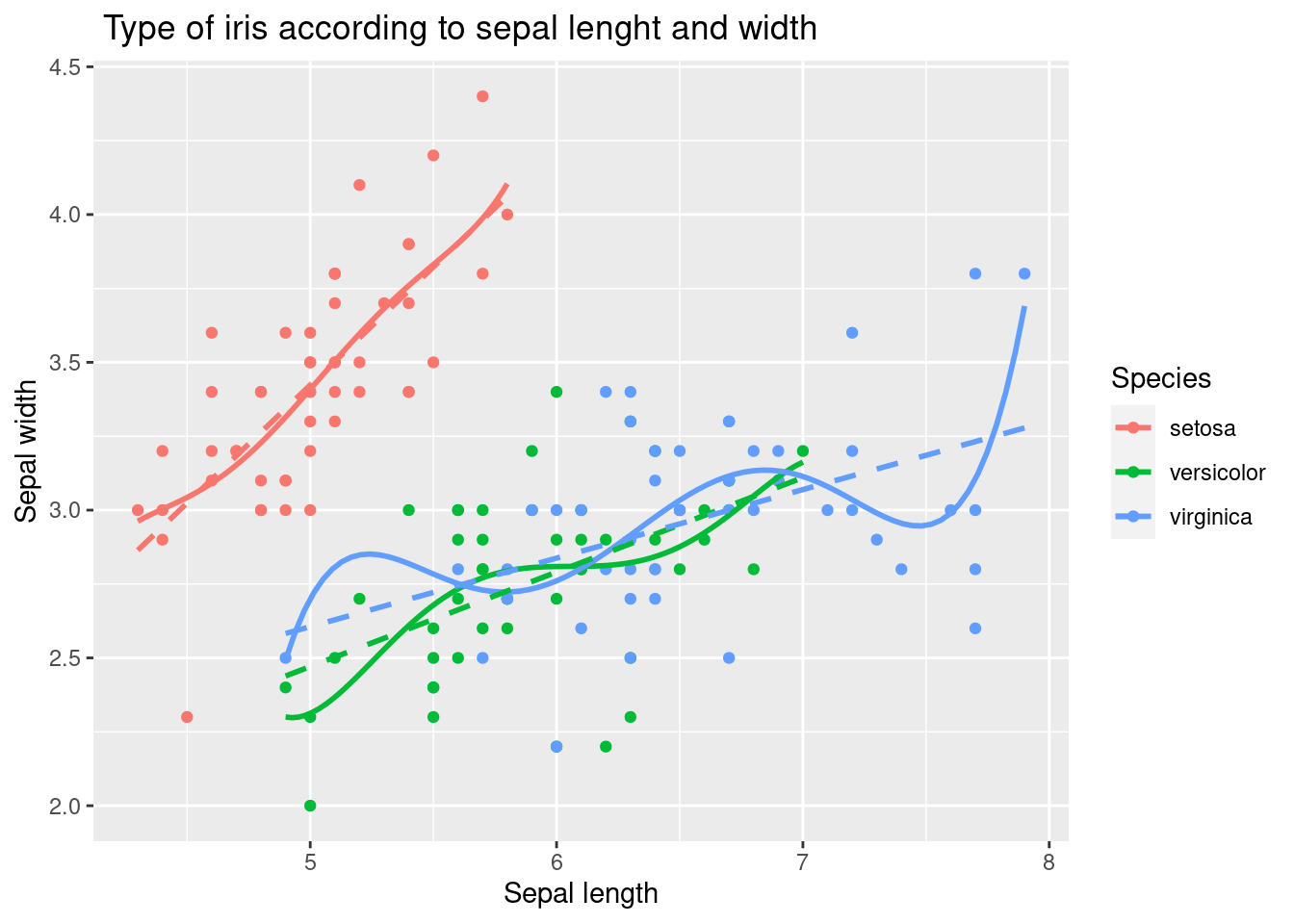
10.1.5 faceting
Drawing on one screen has advantages, but also has complexities. In this case, faceting is used. facet_wrap()
iris %>%
  ggplot(aes(x = Sepal.Length, y = Sepal.Width,
             color = Species)) +
  xlab("Sepal length") +
  ylab("Sepal width") +
  ggtitle(" Type of iris according to sepal lenght and width") +
  geom_point() +
  geom_smooth(method = 'lm', formula = y ~ poly(x, 5), se = FALSE, linetype = 1) +
  geom_smooth(method = 'lm', formula = y ~ x, se = FALSE, linetype = 2)  +
  facet_wrap(Species~.)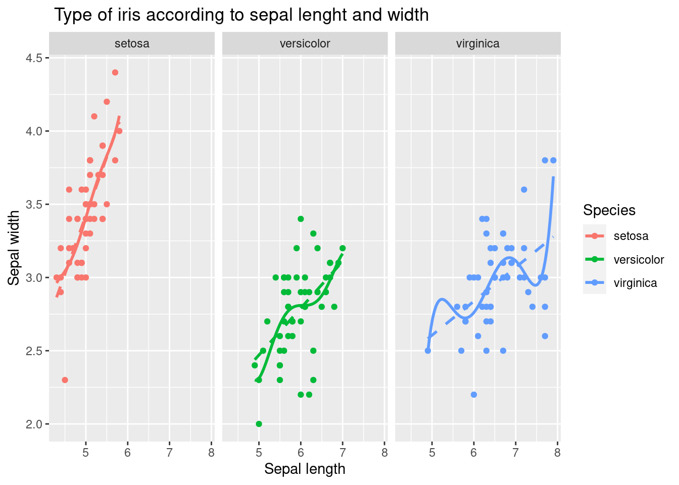
10.1.6 geom_bar()
To make a barplot of counts, we will use geom_bar().
iris %>%
ggplot(aes(x = Species,
fill = Species)) +
xlab("Type of iris") +
ylab("Counts") +
ggtitle("Number of iris according to its types.") +
geom_bar()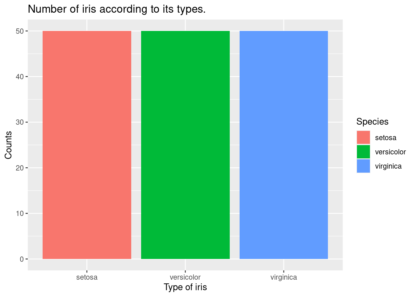 Let’s draw the count number of iris with Sepal.Width equal to or greater than 3. We will use
 filter(Sepal.Width > 3).
iris %>%
  filter(Sepal.Width >3) %>%
  ggplot(aes(x = Species,
             fill = Species)) +
  xlab("Type of iris") +
  ylab("Counts") +
  ggtitle("Number of iris according to its types.") +
  geom_bar()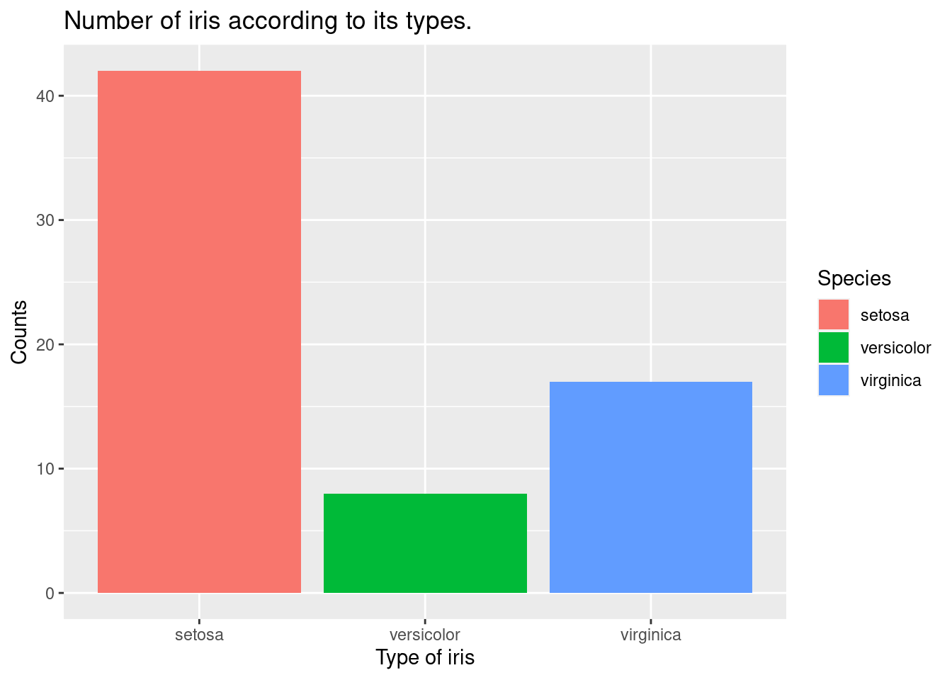
coord_polar is polar coordinate system for pie chart.
iris %>%
  filter(Sepal.Width >3) %>%
  ggplot(aes(x = Species,
             fill = Species)) +
  xlab("Type of iris") +
  ylab("Counts") +
  ggtitle("Number of iris according to its types.") +
  geom_bar() +
  geom_bar(width =1) + coord_polar()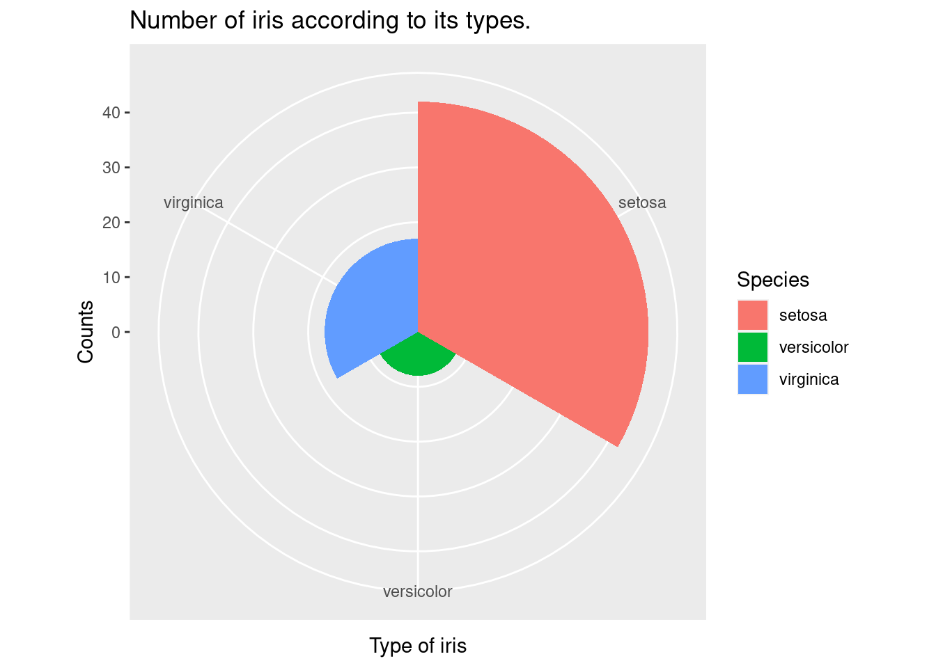
10.1.7 geom_density() , geom_histogram()
Let’s plot the distribution of sepal length. I drew histogram and density.
iris %>%
  ggplot(aes(x = Sepal.Length)) +
  xlab("Sepal Length of Iris") +
  ylab("density") +
  ggtitle("Distribution of Sepal Length ") +
  geom_histogram(aes(y = ..density..))+
  geom_density()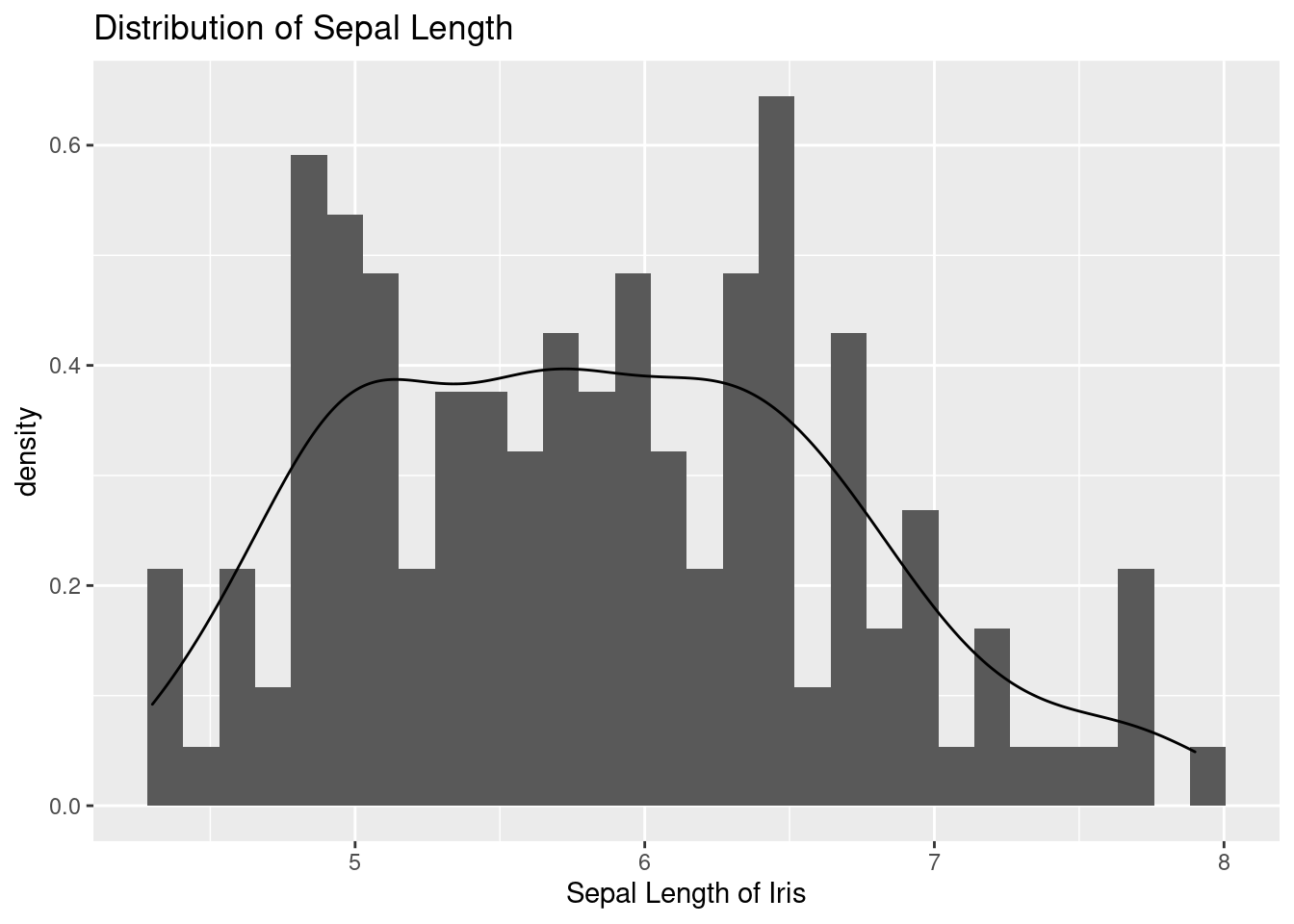
I see heterogeneity. Can you see it. Let’s put fill = Species inside aes() to distinguish them. virginica has broad leaves. How is it different from the previous code of color = Species?
iris %>%
ggplot(aes(x = Sepal.Length, fill = Species)) +
xlab("sepal length of iris") +
ylab("density") +
ggtitle("Distribution of sepal length of iris") +
geom_histogram(aes(y = ..density..), alpha = 0.3)+
geom_density(stat="density", alpha = 0.3) +
theme_minimal()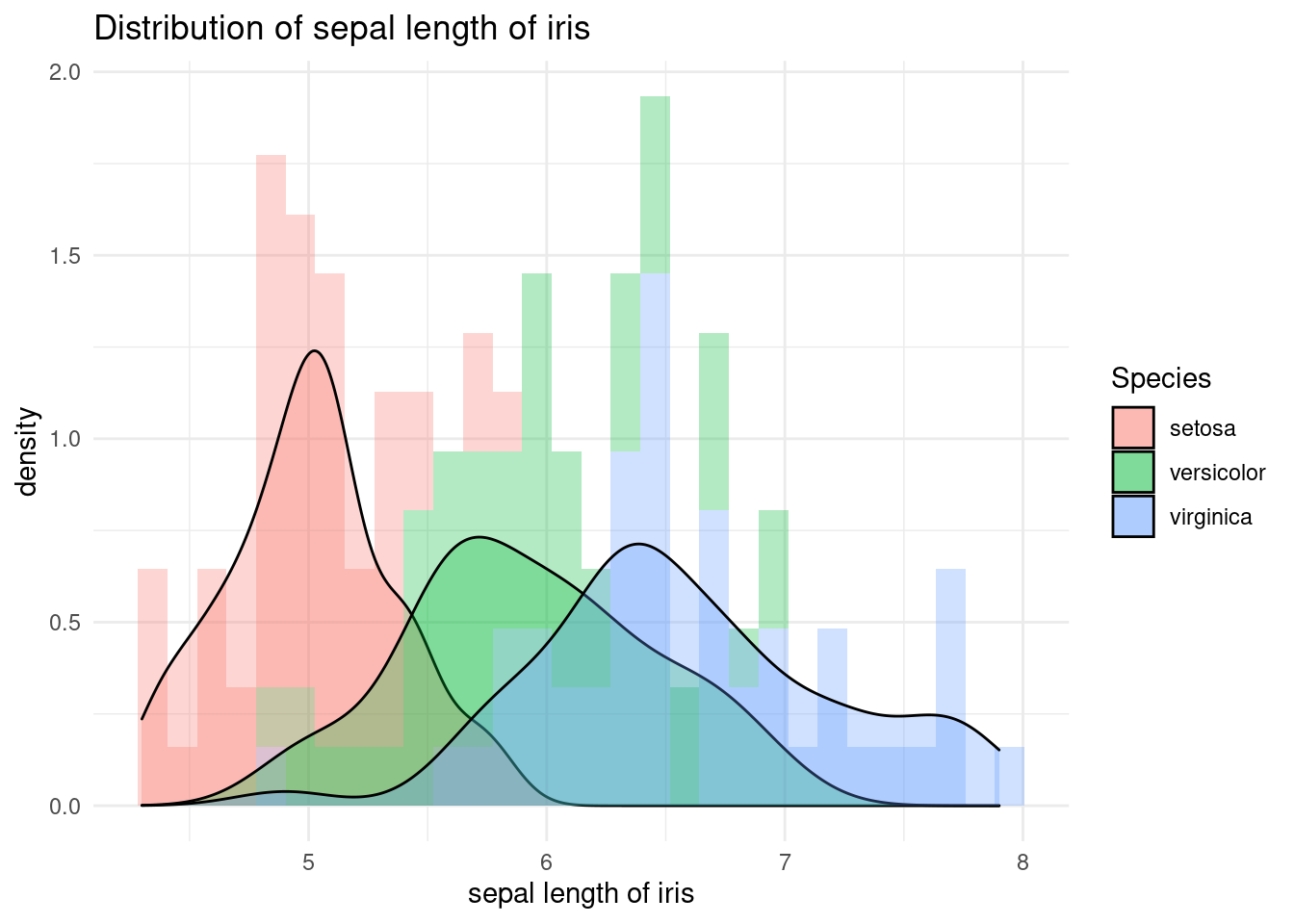 Of course, you can try faceting. Is faceting good in this case? Is it good not to have it? It may be depend on your purpose.
iris %>%
  ggplot(aes(x = Sepal.Length, fill = Species)) +
  xlab("sepal length of iris") +
  ylab("density") +
  ggtitle("Distribution of sepal length of iris") +
  geom_histogram(aes(y = ..density..), alpha = 0.3)+
  geom_density(stat="density", alpha = 0.3) +
  theme_minimal() + # my favorit theme
  facet_wrap(Species~.)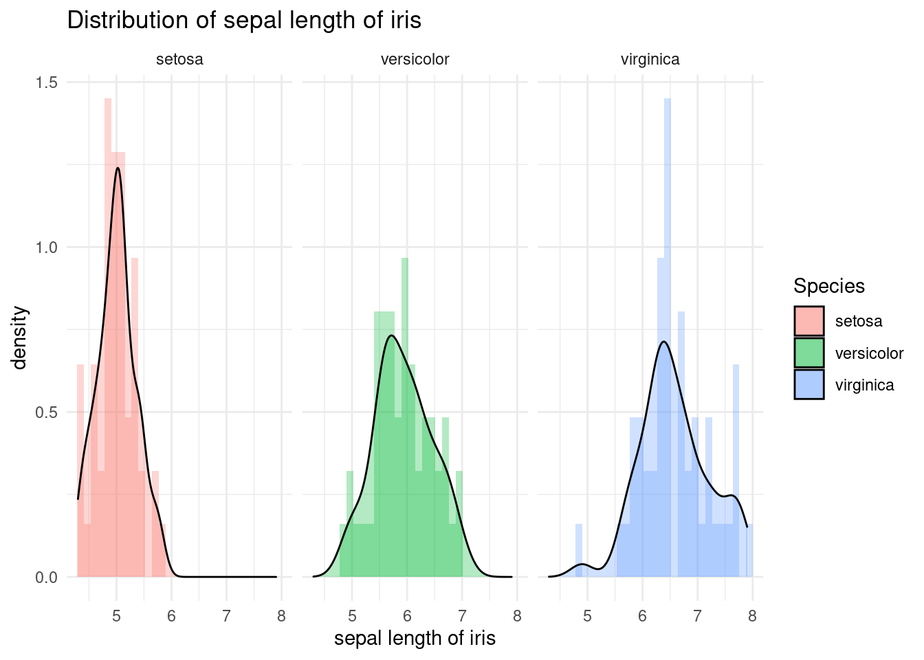
10.1.8 geom_boxplot()
Let’s draw a boxplot of the sepal width distribution for each iris flower.
iris %>%
  ggplot(aes(x = Species, y = Sepal.Width,
             color = Species)) +
  geom_boxplot()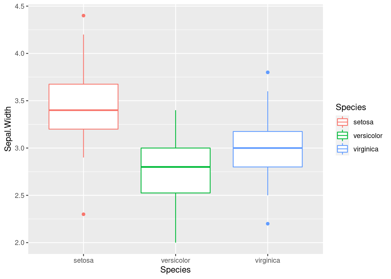
10.1.9 3d plot
In this practice, it seems that the types of iris can be distinguished according to the width and length of the sepals. plot_ly is better than ggplot in interactive part and 3d part. Let’s do it.
library(plotly)
iris %>%
plot_ly(
        x = ~Sepal.Length, y = ~Petal.Length, z = ~Petal.Width,
        color = ~Species,  # Color separation by Species.
        type = "scatter3d",   # 3d plot
        alpha = 0.8
        ) %>%
        layout(
               scene = list(xaxis = list(title = 'Sepal Length'),
                            yaxis = list(title = 'Petal Length'),
                            zaxis = list(title = 'Petal Width')))
10.2 Visualzation example 1
10.2.1 simple machine learning decision tree
Do you think that it is possible to make a decision tree depending on the length and width of the iris? Now that we’ve come this far, let’s just take a look at the flow using simple example. Approximately, decision trees are machine learning methods used for classification. The models aim to predict the value of Y by learning simple decision steps. There are importance weight to make each step of decision. So, it can be visualize bar chart.
10.2.1.1 Divide the data into training and test by 7:3.
I will prepare two data set, one is for training, the other is for testing. The proportion of training set is 70% from original data.
if(!require("caret")) install.packages("caret")
library(caret) #
data(iris)
set.seed(2020)
train_index <- createDataPartition(
           y= iris$Species,
           p = .7,
           list = FALSE,
           times = 1)
train_data <- iris[ train_index,]
test_data  <- iris[-train_index,]
10.2.1.2 10 fold cross validation
Cross-validation is a resampling method for limited data set. I will use 10 fold cross validation.
fitControl <- trainControl(method = "cv", # cross validation
                           number = 10    ) # 10 times
10.2.1.3 machine learning model
check accuracy and model performance using confusion matrix. What is average accuracy for model performance.
set.seed(2020)
DTFit1 <- train(data = train_data, #

                Species ~ ., # . means all remain variable
                method = 'rpart', # https://topepo.github.io/caret/available-models.html
               trControl = fitControl) #  cross validation
confusionMatrix(DTFit1) #
## Cross-Validated (10 fold) Confusion Matrix
##
## (entries are percentual average cell counts across resamples)
##
## Reference
## Prediction setosa versicolor virginica
## setosa 33.3 0.0 0.0
## versicolor 0.0 31.4 1.9
## virginica 0.0 1.9 31.4
##
## Accuracy (average) : 0.9619Our goal is visualization, what kind of plot are needed? The basic bar plot is great choice.
10.2.1.4 barplot for importance
The importance weight differs among variables. Let’s draw importance using bar plot.
fit1_imp <- varImp(DTFit1)
fit1_imp %>%
ggplot(mapping = aes(x = Overall)) +
  geom_boxplot() +
labs(title = "Importance") 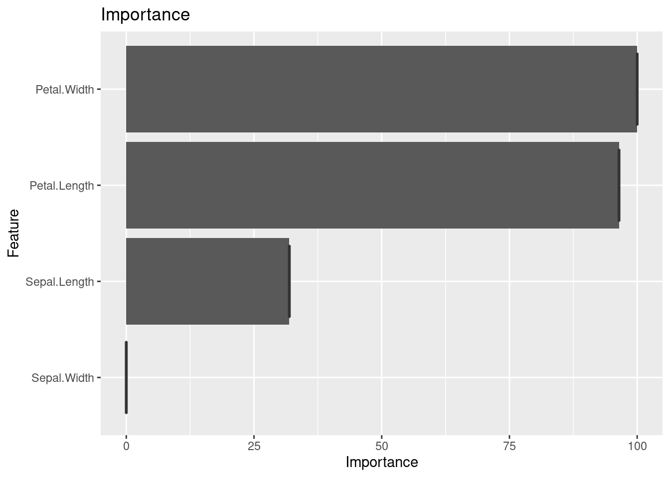
What is most important feature for classification of iris. Petal? Sepal?
rpart package gives us nice plot for decision tree. It can be used for data explorer
library(rpart)
library(rattle)
fancyRpartPlot(DTFit1$finalModel)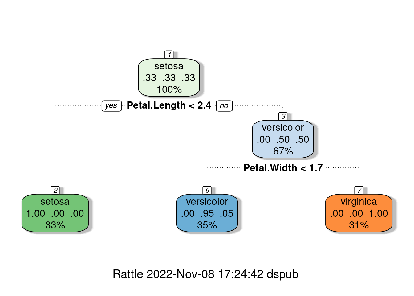
To check this classification steps, we also use 3d plot, as we discussed.